SDR Frequency Tuning Mechanics

This application note discusses the frequency tuning mechanics associated with Per Vices Software Defined Radio (SDR) products for both Tx and Rx functions. Due to the high instantaneous bandwidth of our products, along with tuning ranges that vary between DC to over 18 GHz, our hardware architecture supports various mechanisms to support frequency tuning. The specific mechanisms used for tuning into various frequencies for various device configurations will be discussed, along with expected results.

This application note has been broken down into separate sections for baseband, midband, and highband tuning for both Tx and Rx. The specific frequency range associated with a given tuning methodology is product dependent; we’ve aimed to provide specific ranges here. Though we’ve provided rough operational bounds, please refer to the device product page for authoritative information.

1.Overview

A signal may be shifted (i.e. downconverted/upconverted), either using a mixer, the convertor, or within the FPGA. As each element operates independently of each other, it is possible to shift the frequency at a number of different places, within both the analog and digital domains. This application note discusses the specific tuning mechanisms, along with the relevant frequency mechanics, for each mode of operation (baseband, midband and high-band) for both Tx and Rx.

We use the term Tx mechanics to describe the process by which a low frequency signal is shifted up from baseband, i.e. to an intermediate frequency, that is appropriate for conversion using a digital-to-analog (DAC) converter, before being transmitted via power amplifier and antenna. In this chain, a specific signal path for transmission is selected based on the frequency of the signal (different signal paths are optimized for different frequency ranges). Within each radio chain, the frequency may be mixed by analog or digital mixers, effectively shifting the frequency up to what will be transmitted.

Conversely, we use the term Rx mechanics to describe the process by which a high frequency signal is shifted down from baseband, i.e.to an intermediate frequency, that is appropriate for sampling by a analog-to-digital converter (ADC), as well as the subsequent frequency translations that may occur once the signal is digitized. Referring to Figure 1.1, we see a generalized overview of the frequency mechanics process.

Figure 1.1: Frequency Mechanics Process Overview

2. Baseband Operation

The baseband Tx and Rx chains connect the external SMA input or output to/from the FPGA and converter device through a series RFE amplifiers, filters, mixers, switches, and anti-aliasing or anti-imaging filters. The baseband chain is automatically enabled by configuring the SDR to frequencies below those supported by the analog up/down converter, and within the range shown in Table 1a. The baseband frequency chains do not include any analog mixing stages.

Table 1: Baseband Frequency Bands

Device	Min Frequency	Max Frequency
Crimson	DC	120 MHz
Cyan	DC	500 MHz (may be extended to 800 MHz)

2.1. Baseband Transmit (Tx) Operation

During baseband Tx tuning, the external data port is connected to the FPGA where re-sampling and digital up conversion occur on the FPGA with a CORDIC mixer. There are no analog up- or down- conversion, or mixing stage facilities used when operating in baseband Tx mode.

Baseband Tx Tuning

During Tx operation, data originates from the host user application, passes through the FPGA-based interpolation routine, FPGA-based digital up conversion (using an numerically controlled oscillator (NCO)), before being converted into JESD204B serial data and sent to the DAC. Any user applied frequency shifting occurs after interpolation, prior to sending the JESD serial data to the DAC, as shown in Figure 2.1.1 This also shows the baseband radio front end (RFE) configuration, where the DAC converts the JESD204B data into an analog signal, and passes the signal through anti-imaging filters, before reaching the SMA port which can be connected to a power amplifier and antenna to transmit the signal.

Figure 2.1.1: Baseband Transmission (Tx) Signal Flow

Baseband Tx Mechanics

As the signals progress through the various components/stages of the SDR, the signal’s frequencies and bandwidths that we are dealing with change. Now that we have a good understanding of our circuitry, let’s look at what is happening to the frequency of the signals at each of the SDR stages.

Figure 2.1.2: Baseband Tx Frequency Mechanics

Figure 2.1.2. shows what needs to takes place in our radio to enable the transmission of an analog signal:

1. Data Port Generated Samples: the left side of the image shows three waveforms (A, B and C) that we might be looking to transmit. Prior to the samples getting generated, the user defines a sample rate, which we will call user bandwidth (UBW). The sample rate serves to specify the user bandwidth; an interval [-UBW/2 , UBW/2] which is centred around 0 Hz. Since these waveforms will be offset by the NCO frequency at a later stage, the initial sine waves may (in some cases) have a negative frequency (like signal A in the diagram). Once generated, the samples will be sent to the SDR for further processing. However, it is important to note that sometimes not all of the samples in the user bandwidth will get transmitted (this will become more clear at later stages).
2. Interpolation: after we have generated the user samples, the next step is to perform interpolation used to obtain a larger bandwidth. This new bandwidth specifies a larger interval (also centred around 0 Hz) that is defined by the sample rate of the device (325 MSPS for Crimson TNG, 1 GSPS for Cyan). The user bandwidth is always smaller than the conversion bandwidth. Interpolating the samples to a larger bandwidth is crucial for the next stage where the digital up conversion takes place.

3. Digital Mixing(CORDIC): after interpolating the signal to the conversion bandwidth of the device, the FPGA can proceed to upconvert the samples. Both Crimson TNG and Cyan have CORDIC digital mixers that are capable of both up-conversion and down-conversion (DDC, DUC). Up-conversion is accomplished by mixing the Tx samples with a local oscillator found in the FPGA (set to what is referred to as the NCO frequency). This causes the frequency of all our signals to increase by the NCO frequency. Using the larger conversion bandwidth that we obtained from interpolation ensures that we can capture more of our mixing products. The signals are then serialized and framed via a JESD204B serial link.

   Note

   In some cases, mixing our generated signal with the NCO frequency results in a frequency that does not lie within the user bandwidth. Here the mixing product will still have an image that is rotated, but outside the analog transmit bandwidth: for baseband signals, we discard the negative frequency component (C), so this image isn’t transmitted at the SMA.

4. Digital-to-Analog Converter (DAC): the DAC then converts the serial data to its analog form. The production of images is a fundamental and expected outcome of the Nyquist theorem and so we will still have images of our original signal at each Nyquist zone (i.e. at each multiple of our conversion bandwidth, we are likely to see images of the signal at their corresponding offsets).

5. Anti-Imaging filters: these are used to suppress the images that would typically show up at higher Nyquist zones (multiples of the conversion bandwidth). It has a bandwidth that is ~80% of the DAC bandwidth.
6. RF Gain: the final analog signal now has gain added to it.
7. SMA Edge Launch: the gained analog signal can now be transmitted via power amplifier and antenna.

2.2. Baseband Receive (Rx) Operation

During baseband Rx tuning, the external SMA port is connected to the RFE through a series of amplifiers, filters and switches before reaching the ADC. In addition, re-sampling and digital down conversion occur on the FPGA using an NCO (CORDIC mixer). There are no analog down conversion facilities used when operating in baseband mode. The ADC converts the analog signal to digital, which is then sent to an FPGA which provides framing of the data before being sent over the data port to the host user application.

Baseband Rx Tuning

During Rx operation, a signal originates from the SMA, passes through amplifiers, then anti-aliasing filters, followed by digitization by the ADC into digital JESD204B serial data. This digital signal may then be shifted on either the ADC or FPGA, where is it parsed and passed to the host application over the Ethernet ports. Any user applied frequency shifting occurs after digitization, but prior to decimation, as shown in Figure 2.2.1.

Figure 2.2.1: Baseband Receiver (Rx) Signal Flow

For reception (SDR to user application), the receiver data flow is a mirror of the transmit data-flow we previously discussed. The analog signal incident to the SMA is amplified through a low noise amplifier (LNA), passes through an anti-aliasing filter, and is sampled at the ADC input channel. The digital signal is then passed to the FPGA, where it undergoes digital down conversion using an NCO (CORDIC), and then decimation, prior to being sent to the user application. During receive operation, frequency shifting occurs only prior to decimation.

Baseband Rx Mechanics

Figure 2.2.2: Baseband Rx Frequency Mechanics

Figure 2.2.2 shows what needs to takes place in our radio to receive an analog signal:

1. RF Input/Gain: the first part of the image (see left) shows several pure sine waves (A-E) as they are picked up by the antenna and pass through initial gain amplifier.
2. Lowpass Filter: a low pass filter cuts off any frequencies above a threshold (product dependent).
3. Anti-aliasing filter: an analog anti-aliasing filter aims to restrict the incoming signal to only those that fall in the converter’s bandwidth (an AAF is ~80% of the converter bandwidth). This is important because the ADC’s capture bandwidth is limited by the fixed sampling rate; signals outside the capture bandwidth would otherwise be aliased back into the digitized signal, which would be undesirable. The converter bandwidth specifies a large interval centred around 0 Hz that is defined by the sample rate of the device (325 MSPS for Crimson TNG, 1 GSPS for Cyan). We will shrink our reception interval in later stages so that we only capture the signals we are “tuned” to.
4. Analog-to-digital converter (ADC): this converts the incoming signals into a digital form.
5. Digital Mixing (CORDIC): at this point, the converter BW is large. To prepare for decimation, the samples are digitally down-converted. This decreases the frequency of all the signals from the CORDIC mixer on the FPGA. Both Crimson TNG and Cyan have CORDIC digital mixers that are capable of both up-conversion and down-conversion (DDC, DUC). Down-conversion is accomplished by mixing the Rx samples with a local oscillator found in the FPGA (set to what is referred to as the NCO frequency). Note that after this takes place, some of the frequencies might be negative.
6. Decimation: prior to the samples being received, the user defines a sample rate (call it user bandwidth). The sample rate specifies this user bandwidth (UBW), an interval [-UBW/2 , UBW/2] which is centred around 0 Hz. Decimation ensures that all the incoming signals fall within the user bandwidth.
7. Application: the sampled data can now be sent over Ethernet as frames and used for a specific application.

3. Midband Operation

The midband Tx and Rx chain connects the external SMA input or output to/from the FPGA and converter device through the RFE containing amplifiers, filters, mixers, switches, and anti-aliasing or anti-imaging filters. The midband chain is automatically enabled by configuring the SDR frequencies within the midband range, shown in Table 2 below.

Table 2: Midband Frequency Bands

Device	Min Frequency	Max Frequency
Crimson	120 MHz	6000 MHz
Cyan	500 MHz	6000 MHz

When compared to the baseband signal flow, there are two notable differences:

1. The converter devices operate in dual channel mode to support complex (IQ) operation. Unlike the baseband case, this avoids discarding negative frequency (or the imaginary component) from samples.
2. The RFE includes a complex, analog, mixing stage.

3.1. Midband Transmit (Tx) Operation

Midband Tx Tuning

During midband Tx operation, data originates from the host user application, passes through the FPGA-based interpolation routine, FPGA-based digital up conversion (using an NCO), before being converted into JESD serial data and sent to the DAC. Any user applied frequency shifting occurs after interpolation, prior to sending the JESD204B serial data to the DAC, as shown in Figure 3.1.1. This figure also shows the baseband radio front end (RFE) configuration, where the DAC converts the JESD204B data into an analog signal, and passes the signal through anti-imaging filters, IQ upconverter/complex mixer, before reaching the SMA port which can be connected to a power amplifier and antenna to transmit the signal.

Figure 3.1.1: Midband Transmission (Tx) Signal Flow

Midband Tx Mechanics

Figure 3.1.2 shows what needs to takes place in our radio to enable the transmission of an analog signal in midband. Note how negative frequencies are preserved after the interpolation/complex digital mixing.

Figure 3.1.2: Midband Tx Frequency Mechanics

1. Data Port Generated Samples: the left side of the image shows three waveforms (A,B and C) that we might be looking to transmit. Prior to the samples getting generated, the user defines a sample rate, which we will call user bandwidth (UBW). The sample rate serves to specify the user bandwidth; an interval [-UBW/2 , UBW/2] which is centred around 0 Hz. Since these waveform will be offset by the NCO frequency at a later stage, the initial sine waves may (in some cases) have a negative frequency (like signal A in the diagram). Once generated, the samples will be sent to the SDR for further processing. However it is important to note that sometimes not all of the samples in the user bandwidth will get transmitted (this will become more clear at later stages).
2. Interpolation: after we have generated the user samples, the next step is to perform interpolation to obtain a larger bandwidth. This new bandwidth specifies a larger interval (also centred around 0 Hz) that is defined by the sample rate of the device (325 MSPS for Crimson TNG, 1 GSPS for Cyan). The user bandwidth is always smaller than the conversion bandwidth. Interpolating the samples to a larger bandwidth is crucial for the next stage where the digital up-conversion takes place.

3. Digital Mixing(CORDIC): after interpolating the signal to the conversion bandwidth of the device, the FPGA can proceed to upconvert the samples. Both Crimson TNG and Cyan have CORDIC digital mixers that are capable of both up-conversion and down-conversion (DDC, DUC). Up-conversion is accomplished by mixing the Tx samples with a local oscillator found in the FPGA (set to what is referred to as the NCO frequency). This causes all the frequency of all our signals to increase. Using the larger conversion bandwidth that we obtained from interpolation ensures that we can capture more of our mixing products. (The squiggly line on the frequency axis indicates that the signals (A,B and C) are actually shifted to a much higher bandwidth, and the diagram is for illustrative purposes only).

   Note

   In some cases, mixing our generated signal with the NCO frequency results in a frequency that does not lie within the user bandwidth. Here the mixing product will still have an image that is rotated to fit within our capture bandwidth.

4. Digital-to-analog Converter (DAC): the DAC then converts the signals to their analog form. The production of images is a fundamental and expected outcome of the Nyquist theorem and so we will still have images of our original signal at each Nyquist zone (i.e. at each multiple of our conversion bandwidth, we are likely to see images of the signal at their corresponding offsets).

5. Anti-Imaging filters: these are used to suppress the images that would typically show up at higher Nyquist zones (multiples of the conversion bandwidth). It has a bandwidth that is ~80% of the DAC bandwidth.
6. Analog (IQ) Upconverter/Mixer: this mixer shifts the signals to a higher frequency (upconverts the signal with a frequency synthesizer that generates an LO) at a much greater bandwidth than the converter, and is complex.
7. RF Gain: the final analog signal has gain added to it. (The squiggly line on the frequency axis indicates that the signals (A,B and C) are actually shifted to a much higher bandwidth, and the diagram is for illustrative purposes only).
8. SMA Edge Launch: the gained analog signal can now be transmitted via power amplifier and antenna.

3.2. Midband Receive (Rx) Operation

During midband Rx tuning, the external SMA port is connected to the RFE through a series of amplifiers, filters and switches before reaching the ADC. In addition, re-sampling and digital down conversion occur on the FPGA using an CORDIC mixer. There is further analog down conversion facilities used when operating in midband mode. The ADC converts the analog signal to digital, which is then sent to an FPGA which provides framing of the data before being sent over the data port to the host user application.

Midband Rx Tuning

During midband Rx operation, a signal originates from the SMA, goes through a low-pass filter, before passing through amplifiers, then anti-aliasing filters, followed by digitization by the ADC into digital IQ pairs and transmitted using JESD204B serial data protocol. This digital signal may then be shifted on either the ADC or FPGA, where is it parsed and passed to the host application over the Ethernet ports. Any user applied frequency shifting occurs after digitization, but prior to decimation, as shown in Figure 3.2.1.

Figure 3.2.1: Midband Receiver (Rx) Signal Flow

Midband Rx Mechanics

Figure 3.2.2: Midband Rx Frequency Mechanics

Figure 3.2.2 shows what needs to takes place in our radio to receive an analog signal.

1. RF Input/Gain: the first part of the image (see left) shows several pure sine waves (A-E) as they are picked up by the antenna and passing through an initial gain amplifier.
2. Low-pass Filter: the LPF then cuts off and attenuates all signals above 6GHz.
3. Analog RF Mixer: the signal is then further downconverted using a frequency synthesizer (generates an LO). (The squiggly line on the frequency axis indicates that the signals (A,B and C) are actually shifted to a much lower bandwidth, and the diagram is for illustrative purposes only).
4. Anti-aliasing filter: an analog anti-aliasing filter aims to restrict the incoming signals to only those that fall in the converter’s domain (AAF bandwidth is ~80% that of the ADCs). This is important because the ADC has a finite operating range. The converter bandwidth specifies a large interval centred around 0 Hz that is defined by the sample rate of the device (325 MSPS for Crimson TNG, 1 GSPS for Cyan). We will shrink our reception interval in later stages so that we only capture the signals we are “tuned” to.
5. Analog-to-Digital Converter (ADC): this converts the incoming signals into a digital form.
6. Digital Mixing (CORDIC): at this point, the converter BW is large. To prepare for decimation, the samples are digitally down-converted. This decreases the frequency of all the signals by the NCO frequency set on the FPGA. Both Crimson TNG and Cyan have CORDIC digital mixers that are capable of both up-conversion and down-conversion (DDC, DUC). Down-conversion is accomplished by mixing the Rx samples with a local oscillator found in the FPGA (set to what is referred to as the NCO frequency). Note that after this takes place, some of the frequencies might be negative. (The squiggly line on the frequency axis indicates that the signals (A,B and C) are actually shifted to a much lower bandwidth, and the diagram is for illustrative purposes only).
7. Decimation: prior to the samples being received, the user defines a sample rate (call it user bandwidth). The sample rate specifies this user bandwidth (UBW), an interval [-UBW/2 , UBW/2] which is centred around 0 Hz. Decimation ensures that all the incoming signals fall within the user bandwidth.
8. Application: the sampled data can now be used for a specific application.

4. Highband Operation

To transmit and receive high frequency waves, we need to make use of an additional local oscillator and mixer on the LOgen board. This allows for even higher frequency operation, since our architectures implement a superheterodyne architecture, as discussed on this wikipedia page. This effectively means that the analog frequency conversion is performed in two stages, using a complex base-band stage that is mixed, using an IQ convertor, to a known, real valued IF stage, which is subsequently converted to a final RF stage. The IF stage is implemented using the midband mechanics, as previously discussed in midband mechanics.

The highband Tx and Rx chains connects the external SMA input or output to/from the FPGA and converter device through the RFE containing amplifiers, filters, mixers, switches, and anti-aliasing or anti-imaging filters. The highband chain is automatically enabled by configuring the SDR frequencies within the highband range, shown in Table 3 below.

Table 3: Highband Frequency Bands

Device	Min Frequency	Max Frequency
Cyan	6000 MHz	18000 MHz

4.1. High-band Transmit Operation

Highband Tx Tuning

Figure 4.1.1: Highband Transmission (Tx) Signal Flow

Highband Tx Mechanics

As the samples progress through the various components in the SDR, the frequencies and bandwidths that we are dealing will change. Now that we have a good understanding of our circuitry, let’s look at what is happening to the frequency at each of these steps, as shown in the figure below:

Figure 4.1.2: Tx Highband Mechanics

1. Data Port Generated Samples: the left side of the figure shows three waveforms (A,B and C) from the data port which we want to transmit. Prior to the samples getting generated, the user defines a sample rate, which we will call user bandwidth (UBW). The sample rate serves to specify the user bandwidth; an interval [-UBW/2 , UBW/2] which is centred around 0 Hz. Once the samples are generated, they are sent to the SDR for further processing.
2. Interpolation: after we have generated the user samples, the next step is to perform interpolation used to obtain a larger bandwidth. This new bandwidth specifies a larger interval (also centred around 0 Hz) that is defined by the sample rate of the device (325 MSPS for Crimson TNG, 1 GSPS for Cyan). The user bandwidth is always smaller than the conversion bandwidth. Interpolating the samples to a larger bandwidth is crucial for the next stage where the digital upconversion takes place.
3. CORDIC Mixing: after interpolating the signal to the conversion bandwidth of the device, the FPGA can proceed to upconvert the samples. Both Crimson TNG and Cyan have CORDIC digital mixers that are capable of both up-conversion and down-conversion (DDC, DUC). Up-conversion is accomplished by mixing the Tx samples with a local oscillator found in the FPGA (set to what is referred to as the NCO frequency). This causes the frequency of all our signals to increase. Using the larger conversion bandwidth that we obtained from interpolation ensures that we can capture more of our mixing products. This also produces image signals via image wrap-around (signal C). The production of images is a fundamental and expected outcome of the Nyquist theorem and so we will still have images of our original signal at each Nyquist zone (i.e. at each multiple of our conversion bandwidth, we are likely to see images of the signal at their corresponding offsets). (The squiggly line on the frequency axis indicates that the signals (A,B and C) are actually shifted to a much higher bandwidth, and the diagram is for illustrative purposes only).
4. Digital-Analog-Converter: the DAC then converts this digital signal to analog, which attenuates the image signals significantly.
5. Anti-Aliasing Filter: an AAF is then able to get rid of the image signals, while also decreasing the bandwidth to 80% of the DAC bandwidth.
6. Complex (IQ) Upconverter/Mixer 1: an analog upconverter/mixer is then used to further increase the frequency of each signal, using a midband frequency LO (IF). (The squiggly line on the frequency axis indicates that the signals (A and B) are actually shifted to a much higher bandwidth, and the diagram is for illustrative purposes only).
7. Band-pass Filter: this signal then goes through a BPF, which only permits signals from 1.4 - 2.3 GHz.
8. Passive (Real) Upconverter/Mixer 2: this further upconverts the signal using a highband frequency LO (and is a real valued mixer), and then through a HP filter which rejects signals below 6GHz. (The squiggly line on the frequency axis indicates that the signals (A and B) are actually shifted to a much higher bandwidth, and the diagram is for illustrative purposes only).
9. RF Gain: the final signals which will be transmitted are amplified. (The squiggly lines are to indicate that the signals (A and B) are actually at a much higher bandwidth, and the diagram is for illustrative purposes only).
10. SMA edgelaunch: the gained final analog signal can now be transmitted via power amplifier and antenna.

4.2. Highband Receive Operation

Highband Rx Tuning

Figure 4c: Highband Receiver (Rx) Signal Flow

Highband Rx Mechanics

Figure 4d: Rx Highband Frequency Mechanics

The figure above shows what needs to take place in our radio in order to receive an analog signal.

1. RF Input/Gain: the first part of the figure shows several pure sine waves (A-F) and their images being picked up by an antenna attached the SMA jack and then amplified.
2. High Pass Filter: in this stage, the signals pass through a HPF which attenuates all signals below 6GHz.
3. RF (Real/Passive) Downconverter/Mixer: next the signals reach a mixer (real) which performs frequency down conversion using an high frequency (HF) LO, as shown on the figure above. Note how signal B reflects from the horizontal (0Hz) axis due to this being a real valued mixer.
4. Band Pass Filter: the down converted signals then pass through a BPF, which permits frequencies between 1.4 - 2.3 GHz while attenuating all other frequencies outside this band.
5. Complex (IQ) Downconverter/Mixer: these signals are further downconverted by a mixer (complex), using the IF LO, which then separate the signal into IQ pairs, before each component being filtered further and then amplified.
6. Anti-Aliasing Filter: signals then reach an AAF which are applied to both the I and Q signal, while attenuating signals outside the AAF bandwidth, which is 80% that of the converter bandwidth.
7. Analog-Digital Converter: this converts the signals from analog to digital domain, where the signals are now able to be manipulated on the FPGA.
8. Digital Mixing (CORDIC): this decreases the frequency of all the signals by the NCO frequency set on the FPGA. Both Crimson TNG and Cyan have CORDIC digital mixers that are capable of both up-conversion and down-conversion (DDC, DUC). Down-conversion is accomplished by mixing the Rx samples with a local oscillator found in the FPGA (set to what is referred to as the NCO frequency). Note that after this takes place, some of the frequencies might be negative (signals D and C). Signals that are rotated beyond the convertor boundary, wrap around on the other side of the bandwidth (signals C and D). This operation does not lose any information, it simply rotates the signal in the frequency domain. (The squiggly line on the frequency axis indicates that the signals (C,D, and E) are actually shifted to a much lower bandwidth, and the diagram is for illustrative purposes only).
9. Decimation: this further down samples the signals and dictates the final user bandwidth before proceeding to the host computer/application.
10. Application: the sampled data can now be sent over Ethernet as frames and used for a specific application.

5. Basic Definitions

Below we discuss how one would use the frequency tuning mechanics discussed above in order to transmit or receive a signal. This is done using the mixers, both real/complex analog and complex (CORDIC) digital mixers,as well as decimation. First, a few basic definitions:

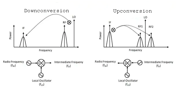
1. Downconversion is the process of mixing an RF input and LO to obtain an output IF lower than the RF input:

   \[ f_{IF}= \mid f_{LO} -f_{RF} \mid \]

2. Upconversion is the process of mixing an LO such that RF output is larger than the RF input:

   \[ f_{RF_1}= f_{LO} - f_{IF} \]
   \[ f_{RF_2}= f_{LO} + f_{IF} \]

   Figure 5a: Downconversion and Upconversion

   

3. The total offset that we wish to shift a signal (i.e. upconvert or downconvert) is defined as follows for each band:

   Baseband: \(f_{offset} = f_{NCO, FPGA}\)

   Midband: \(f_{offset} = f_{LO,MB} + f_{NCO}\)

   Highband: \(f_{offset} = f_{LO,HF} + f_{LO,IF} + f_{NCO, FPGA}\)

4. Decimation refers to the process of reducing the sampling rate (i.e. downsampling) by essentially throwing away samples. The decimation factor (M) is defined as the ratio of the input rate to output rate. In equation form, we have:

   \[ M = \frac {input (SPS)}{output (SPS)} \]

5. Interpolation refers to the process of increasing the sampling rate (i.e.upsampling) by essentially inserting zero valued samples. The interpolation factor (L) is defined as the ratio of the output rate to input rate. In equation form, we have:

   \[ L = \frac {output (SPS)}{input (SPS)} \]

5.1 Glossary of Bandwidth Terminology

Sampling Bandwidth (ADC/DAC Bandwidth): This is the bandwidth at which the converters are operating at. For a single real-valued signal, this corresponds to half the sample rate (by Nyquist’s theorem). For a complex signal (i.e. IQ pairs), this corresponds to the sample rate. This should make sense intuitively; given a fixed sample rate, a complex signal, with its two orthogonal components (i.e. I and Q), carries twice the amount of information than a real valued signal.

Note that when our device operates in baseband mode, we only sample from a single channel (the “I” channel, at 16bits), and convert it to a complex signal by adding a virtual “zero” to the Q channel within the FPGA. As an example, the default Cyan product has a constant sample rate of 1GSPS for all convertor devices and channels. This means that, when operating in baseband mode, our sampling bandwidth corresponds to half the converter sample rate (i.e. 500MHz for Cyan). However, when operating in Mid- or Highband, we use both channels (transmitting/receiving I and Q, each at 16bits), and the product therefore has a sampling bandwidth of 1GHz.

This is an important distinction for two reasons; it provides the theoretical bound on the maximum bandwidth we can send and receive at any given time. It also allows customers who want to bypass the default radio front end, an idea of what kind of analog filtering they would require.

RF Bandwidth (AAF/AIF bandwidth): The RF bandwidth corresponds to the actual radio bandwidth of the product. This is generally the 3dB bandwidth at which we have implemented the analog anti-aliasing filters (AAF) and anti-imaging filters (AIF). In the case of our default Cyan product, this comes to around 800MHz. It’s important to note that this is NOT a brick wall filter since we will be able to observe frequencies past 800MHz, they’ll just be attenuated. Moreover, signals immediately beyond the sampling bandwidth of the ADC/DAC will appear to be reflected about that bandwidth.

Because the analog domain is continuous, there will exist frequencies beyond the sampling bandwidth. By virtue of Nyquist, we know that, once digitized, any frequencies beyond the sampling bandwidth will reflect back on to the signal (i.e. be aliased, in the case of receiving), or be multiplied on the output (imaging, in the case of transmission). Imaging and aliasing are both very undesirable, as it entails that there’s no way to differentiate between, say, a signal that is at 900MHz vs. a signal at 1100MHz. Unless we use analog filtering, the aliasing and imaging can cause serious problems. Particularly this is problematic since the bandwidth of the analog components used in the radio chain are often greater than the sampling bandwidth the convertors are running at. It’s therefore important to match these in order to reduce the impact of aliasing or images.

For example, if you receive a sufficiently strong base band signal, say at 0dBm, at 1100MHz, the RF anti-aliasing filter may attenuate that signal to, -40dBm. However, when sampling that signal at the convertor, you’ll actually see it placed at 900MHz (because the sampling bandwidth is at 1000MHz, and the signal is 100MHz above that, it gets reflected back down to 900MHz). However, the amplitude of this signal as its frequency increases will get increasingly smaller, because the analog anti-aliasing filter will have stronger rejection as the input signal frequency increases beyond the passband (which we’ve set to 800MHz). As a general rule of thumb, we define the pass band as 80% of the total sampling bandwidth, and it’s usually reserved for the filter’s roll off/transition band.

We use 80% because designing analog filters is hard. Ideally, we want to have a flat pass band, and super steep rejection (i.e. a very small “transition band”) to the “stop band” value. For example, a flat, say, -2dB insertion loss within the pass band, but then immediately outside of it, -60dB of stop band attenuation. The general problem here is that having a steep/small transition bandwidth limits the maximum stop band attenuation. Which is to say, we could have a much steeper transition band, but then the attenuation of signals may be insufficient to prevent aliasing/meet the SNR/SFDR requirements of the system. We picked an 80% value because it helps ensure that the stop band attenuation is sufficiently high so as to match the overall SNR/SFDR requirements of the system (targeted at 40-60dB).

Application Bandwidth (User Bandwidth): Everything we’ve mentioned above reflects fixed architectural characteristics of the clocking configuration and radio front end chains. It also impacts the fixed link between the FPGA and the convertor device. However, once the data is on the FPGA, we provide the ability to either interpolate data upwards to a sample rate (in the case of transmitting information from the SDR), or decimate it down to a lower sample rate (in the case of sending information). This is accomplished through Digital Up Conversion (DUC; for sending info from the SDR), or Digital Down Conversion (DDC; to receive data from SDR). As these filters are implemented digitally, we can use substantially longer taps (i.e. co-efficient) than what would commercially and economically be possible using analog components. This means our filters can have more ideal behaviour. It also provides customers with the ability to select more convenient sample rates depending on their actual application. Provided that the input sample rate is an integer multiple (or divisor) of the fixed sample rate of the device (1GSPS for Cyan/ 325MSPS for Crimson), then the SDR is capable of handling the matching between the rate at which the application or user sends/receives information, and the rate at which the FPGA is sending/receiving information to/from the converter.

6.Tuning Mechanics Examples

This is a collection of examples to illustrate the above concepts.

6.1 Crimson Baseband Tx Tuning

Problem: We are looking to transmit a 1MHz sine wave, to a center frequency of 60MHz. What is a reasonable sample rate, DSP frequency, and LO frequency to accomplish this?

Solution: Since the center frequency is 60MHz we can use the baseband for transmission.

1. Data Port Generated Samples: the left side of the image shows the waveform A to be transmitted. Since we need to transmit 1MHz sine wave consider the oversampling of x8 = 8MSPS

2. Interpolation: This new bandwidth specifies a larger interval (also centred around 0 Hz) that is defined by the sample rate of the device (325 MSPS for Crimson TNG, 1 GSPS for Cyan).

3. Digital Mixing(CORDIC): The NCO frequency is adjusted to +59MHz offset in order to center the signal at 60MHz.Since there are no analog mixing stages for baseband the LO tuning frequency is set to 0.

4. Digital-to-Analog Converter (DAC): the DAC then converts the serial data to its analog form. The production of images is a fundamental and expected outcome of the Nyquist theorem and so we will still have images of our original signal at each Nyquist zone (i.e. at each multiple of our conversion bandwidth, we are likely to see images of the signal at their corresponding offsets).

5. Anti-Imaging filters: these are used to suppress the images that would typically show up at higher Nyquist zones (multiples of the conversion bandwidth). It has a bandwidth that is ~80% of the DAC bandwidth(~260MHz for crimson and ~800MHz for cyan).

6. RF Gain: the final analog signal now has gain added to it.

7. SMA Edge Launch: the gained analog signal can now be transmitted via power amplifier and antenna.

6.2 Crimson Baseband Rx Tuning

Problem: We are looking to receive a 1MHz sine wave being receiving at a 50MHz center frequency. What is a reasonable sample rate and DSP frequency and what is the frequency of the final tone?

Solution:The baseband Rx can be used since the center frequency is 50MHz.

1. RF Input/Gain: The first part shows the sine wave being received at center frequency of 50MHz.

2. Lowpass Filter: a low pass filter cuts off any frequencies above a threshold (for Crimson any frequency above 120MHz for baseband).

3. Anti-aliasing filter: an analog anti-aliasing filter aims to restrict the incoming signal to only those that fall in the converter’s bandwidth (an AAF is ~80% of the converter bandwidth).

4. Analog-to-digital converter (ADC): this converts the incoming signals into a digital form.The converter bandwidth specifies a large interval centred around 0 Hz that is defined by the sample rate of the device (325 MSPS for Crimson TNG, 1 GSPS for Cyan).

5. Digital Mixing (CORDIC):The NCO frequency is then adjusted to downconvert the signal to receive an output of 1MHz. The desired offset in this case is 49MHz. The LO tuning word is set to 0 since there are no analog mixers in the baseband.

6. Decimation: The sampling rate is set to 8MSPS for the specified frequency of 1MHz.

7. Application: the sampled data can now be sent over Ethernet as frames and used for a specific application.

6.3 Crimson Rx and Tx Midband Tuning

Problem: Our application generates a complex signal with a final bandwidth of 32.5MHz, and we are looking to transmit this signal to a center frequency of 5025MHz. To test our work, we are going to loop the signal back to the Rx port, through a 30dB attenuator, and sample a pilot tone at 1MHz, that is located at a -5MHz offset of center of the transmitted signal. Our \(f_{LO, MB}=N*100\) MHz, where N is a whole number and the DAC has a sample rate of 325MSPS. What would be reasonable values for our \(f_{NCO,FPGA}\), and \(f_{LO, MB}\), for both Rx and Tx, along with a reasonable Rx sample rate?

Solution: Crimson Tx Midband Tuning

1. Data Port Generated Samples: The left side represents the signal B at 32.5MHz(user defined) bandwidth to be transmitted

2. Interpolation: Next stage represents interpolating the samples to larger bandwidth for up conversion.This new bandwidth is defined by the sample rate of the device (325 MSPS for Crimson TNG).

3. Digital Mixing(CORDIC): During this stage the FPGA NCO frequency is provided. In this case since we need to transmit the signal to a center frequency 5025MHz

   \(f_{offset} = f_{LO,MB} + f_{NCO}\)

   offset = 5025 - 32.5 =4992.5

   provided \(f_{LO, MB}=N*100\) select N as 49

   f_{LO,MB} = 4900MHz

   f_{NCO} = 92.5MHz

4. Digital-to-analog Converter (DAC): the DAC then converts the signals to their analog form. The production of images is a fundamental and expected outcome of the Nyquist theorem and so we will still have images of our original signal at each Nyquist zone (i.e. at each multiple of our conversion bandwidth, we are likely to see images of the signal at their corresponding offsets).

5. Anti-Imaging filters: these are used to suppress the images that would typically show up at higher nyquist zones (multiples of the conversion bandwidth). It has a bandwidth that is ~80% of the DAC bandwidth.

6. Analog (IQ) Upconverter/Mixer: This mixer uses the above calculated LO frequency to further upconvert the signal to required center frequency of 5025MHz.

7. RF Gain: the final analog signal has gain added to it.

8. SMA Edge Launch: the gained analog signal can now be transmitted via power amplifier and antenna.

Crimson Rx Midband Tuning

1. RF Input/Gain: the first part shows the signal B centered at 5020MHz(-5 offset of center of transmitted signal).

2. Low-pass Filter: the LPF then cuts off and attenuates all signals above 6GHz.

3. Analog RF Mixer: the signal is then further downconverted using a frequency synthesizer (generates an LO).We need to sample a pilot tone of 1MHz,

   f_offset = 1-5020 = -5019

   \(f_{LO, MB}=N*100\) MHz

   Select N = 50

   f_{LO, MB} = 5000MHz

   f_{NCO} = 19MHz

4. Anti-aliasing filter: an analog anti-aliasing filter aims to restrict the incoming signals to only those that fall in the converter’s domain (AAF bandwidth is ~80% that of the ADCs).

5. Analog-to-Digital Converter (ADC): this converts the incoming signals into a digital form.

6. Digital Mixing (CORDIC): This stage sets the FPGA NCO bandwidth as f_{NCO}= 19MHz

7. Decimation: prior to the samples being received, the user defines a sample rate in this 8MSPS(oversampling factor x8) for receiving a sample pilot of 1MHz.

8. Application: the sampled data can now be used for a specific application.

6.4 Cyan Baseband Rx Baseband

Problem: Suppose you are looking to analyze a 1MHz QPSK signal, centered at 40MHz, with a desired application BW of 2MHz. What are the tuning parameters to achieve this?

Solution:

1. Understand the goal and information given in the question

   Goal: Shift signal down to zero, so it is within the 2 MHz desired bandwidth

   Information: In this question we are understanding 1 MHz to be the span of the QPSK signal, so the bandwidth is 1 MHz and it is surrounding 40 MHz.

2. Understand the Cyan Baseband Operation

   The baseband operation only has one mixer, the FPGA. This means there is only one frequency requirement: the NCO. *Note: There are filters you may have to consider when sending signals to this band, but this question does not run into that issue. Refer to Rx Baseband Operations *

3. Mathing out the Parameters

   Parameter	Description	Math	Explanation
   Sample Rate	Number of samples taken per seconds	\(Sample Rate \times Over Sampling Ratio\) \(1 MHz \times 8 = 16 MSPS\)	The minimum sampling rate is equal to the bandwidth because the units work in the complex domain. Then, to ensure we get clear readings, we multiply the minimum sampling rate by an oversampling ratio. Here 8 was chosen.
   Frequency Offset/Shift	The total shift the mixers must do to ensure the signal ends up at the right frequency.	\(Answer: 40 MHz\)	As there is only one mixer in the baseband, the total shift is equivalent to the input centre.

Figure 6.4: Solution Diagram

6.5 Cyan Baseband Tx Tuning Example

Problem: Now let’s say you are looking to generate a sinewave at 300 MHz Solution:

1. Understanding the Goal and information

   Goal: Shift a signal up to 300 Mhz

   Information: Since we are generating the signal, we are going from digital to analog and shifting the signal up.

2. Understanding the Unit

   This signal will go through the baseband, so it is a similar process to the previous example. However, there is a slight change in the process due to DC blocking, otherwise it is very similar to the last problem.

   DC Blocking: Dc Blockers are circuit components that essentially block 0 Hz digital waves. The reason they exist are to prevent interference with other radio frequencies. This effects you because it means you can’t shift your digital signal to 0, so people often use offsets. They are essentially an arbitrary value away from zero to generate your frequency.

3. Mathing out the parameters

   Parameter	Description	Math	Explanation
   Wave Frequency	Initial frequency your signal will start with. Confusingly, this is called the offset sometimes.	2 MHz	This is just an easy value to work with.
   Sample Rate	The total shift the mixers must do to ensure the signal ends up at the right frequency.	\(Sample Rate \times Over sampling ratio\) \(\Rightarrow Sample Rate = 2 MHz \times 2\) \(\Rightarrow 4 MHz \times 8 = 32 MSPS\)	The minimum sample rate of a 2 MHz sinewave is 4 MHz because there has to be at least two samples per cycle. Then, you multiply by the over sampling rate.
   Frequency Offset/Shift	Initial frequency your signal will start with.	\(70 MHz - 2 MHz = 68 MHz\)	This is just an easy value to work with.

6.6 Cyan Highband Rx Tuning Example

Problem: You are looking to receive a 5MHz FM chirp at a center frequency of 12.56GHz. What is a reasonable sample rate, and tuning frequencies to accomplish this?

Solution:

1. Understanding the Goal and information

   Goal: Shift a signal received at 12.56GHz down to 0 (remember: since we are changing this frequency to digital, we can shift to 0).

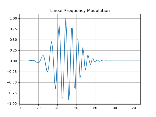
   Information: It’s important to always understand what sort of signals we are receiving. Chirps aren’t a periodic signal like the previous two examples, so we work with it a little different. Below is a frequency-time graph roughly explaining what the chirp looks like. For this question, let’s assume it’s a linear movement from zero to 5 MHz. Notice how this means the bandwidth is 5 MHz.

   Figure 6.7.1: Chirp Diagram

   

   These differences mean you could either shift your signal to start at 0 or be centered at 0. Starting at 0 is the same as the process in 6.4. Centering at 0 requires you to add 0.5 of the chirp to the offset as you are down converting. For this question, assume you must receive it centered at zero.

2. Understanding the Unit

   This signal goes through the Highband operation. This means there three frequency parameters that must be set: LO HF, LO IF, and NCO. They represent two mixers and the FPGA. The total offset is found the same way as previous questions, but the value must properly be allotted between the three frequencies.

3. Mathing out the parameters

   Parameter	Description	Math	Explanation
   Sample Rate	Initial frequency your signal will start with. Confusingly, this is called the offset sometimes.	\(Sample Rate \times Over sampling ratio\) \(\Rightarrow 4 MHz \times 8 = 32 MSPS\)	Because this is a complex signal, the sample rate is equivalent to bandwidth.
   Frequency Offset/Shift	The total shift the mixers must do to ensure the signal ends up at the right frequency.	\(12560 MHz + (0.5 \times 5 MHz) = 12562.5 MHz\)	This is equivalent to the centre frequency because we can down convert to 0. The value also has been converted to MHz for simplicity
   Frequency of LO IF	Frequency of the intermediate frequency local oscillator.	1800 MHz	In only the highband, this mixer has a fixed frequency.
   Frequency of LO HF	Frequency of the high frequency local oscillator.	\(12562.5MHz - 1800 MHz = 10762.5\) \(\Rightarrow Frequency_{LO HF} = 10700 MHz\)	Found how much more the frequency has to shift by, then noted the Cyan unit’s LO can only step in multiples of 100.
   Frequency of NCO	Frequency of the FPGA.	62.5 MHz	Found from the “left over” of the other frequencies.

Refer to diagram below to understand what is happening:

Figure 6.6: Solution Diagram

6.7 Crimson Midband Tx Tuning Discussion

Analog Domain

From the SMA (RF Input), the RF signal is down-converted in the analog domain by the RF (IQ) mixer. At this point, two low pass filters (LPF) (one for I and one for Q), serve to attenuate any other RF signal outside this bandwidth. Within the complex domain, this corresponds to +/- 120Mhz (for 240 MHz about DC, which, because this is a direct IQ down converter, would corresponds to whatever frequency you set the LO to.

The down convertor is subject to some limitations, including image rejection about that 240 MHz band, which is typically around -40dB. As these images are, by definition, within the pass band of the low pass filter, they are present within the bandwidth of the analog signal.

So, if injecting a 2.8 GHz signal, and setting the LO to 2.7GHz, after IQ down-conversion, the complex spectrum (don’t think about the real valued one for now), would contain your fundamental at +100MHz, say, at 0dBm, and the image at -100MHz, at, say, -40dBm. As both of these signals fall within pass band of +/-120MHz, they actually exist within the analog signal bandwidth and will, by extension, exist in the sampled signal bandwidth (i.e. ADC bandwidth).

Digital Domain

From there, the digitized signal is shifted by the NCO. Mathematically, this occurs in a discrete and periodic space, whose period corresponds to the sample rate. Again, because this is a complex transform, the Nyquist criteria works out so that the magnitude of the bandwidth corresponds to the sample rate.

When using the NCO, it shifts all frequencies within the sample bandwidth of 325MHz. So, continuing the above example, using the NCO to shift the effective IF by -100MHz (thereby shifting the relative frequency of the fundamental from +100MHz to 0Hz in the complex spectrum), also results in the image, which used to be at -100MHz, being shifting to +125MHz.

This happens as follows; The total complex bandwidth of 325MHz is centred about 0Hz, with boundaries at +/-162.5MHz. The image is initially located at -100MHz relative to the 0Hz center frequency. When we shift the image by -100MHz (in order to center the fundamental tone), we also need to shift the image by the corresponding amount. In order to shift the image by -100MHz, we first shift the image by -62.5MHz, which brings us the lower bound of -162.5MHz, and results in us wrapping around to +162.5MHz, with an additional -37.5MHz shift to go. Applying the -37.5MHz balance of the -100MHz shift (-62.5MHz + -37.5MHz = -100MHz) from the top moves the image to +125MHz. So now, after conversion and the frequency shift of the NCO, we have our fundamental centred at 0Hz, and the original IQ image at +125MHz.

Next, comes decimation. This process is a bit complex, but basically comes down to first applying a low pass filter on both the I and Q streams (which corresponds to a band pass filter centred about 0Hz in the complex domain), and then decimating by the required amount.

So if we aim to decimate the bandwidth to, say, 10MHz, and our fundamental is still centred on 0Hz, and the image is at +125MHz, this corresponds to first applying a 5MHz low pass filter on both the I and Q streams, which is equivalent to applying a 10MHz band pass filter centred about 0Hz on the complex stream with a bandwidth of 325MHz.

This band pass filter attenuates any signal outside the 10MHz band centered about 0Hz, which happens to include our image at +125MHz. Only after filtering does the actual decimation (i.e. removing dropped samples from the digital stream) occur.

As a practical matter, the greater the amount of decimation, the narrower the band pass filters are, and the greater the attenuation of any images. In addition, the further from the stop band frequencies, the greater the attenuation. However, for the purposes of this very specific application and discussion, the filters work exceedingly well to attenuate any out of band images, with stop band attenuation close to the 96dB dynamic range limitation associated with 16-bit integers.

Takehome message

1) The FPGA NCO chain or decimation change do not introduce any (unexpected) artifacts or harmonics into the digital stream. For the frequency ranges we’ve discussed above, the signals observed for a given NCO shift are actually present in the signal. (This does not necessarily hold when operating close to the ADC sample rate of 162.5MHz, in which case you will see aliasing, but, given the example above, this should not be an issue).

2) Although it’s convenient to consider the FPGA NCO as operating as a mixer, this is not entirely true. When we discuss mixing, it’s actually implemented as a CORDIC, with an internal phase resolution of 32bits, implemented as a 20th order series, and includes correction factors to ensure spur reduction. The end result is that the mode of operation for the NCO is fundamentally different than that of an analog mixer. As we’ve implemented a mathematical transform, it doesn’t add spurs.