Building an FM Receiver with gnuradio
By the end of the tutorial, you will be able to put together a FM radio broadcast receiver that operates like the ones found in most cars. This is a good way to verify that the Rx channels on your Crimson TNG / Cyan are working and will help you get started with gnuradio.
In this tutorial, we will cover:
- A big picture overview of how FM Broadcast works
- What a typical workflow is like with gnuradio
- How to make sure your Crimson TNG / Cyan works with your gnuradio installation
Note
Before embarking on this tutorial, you’ll want to setup your Crimson TNG or Cyan radio.
Requirements
Hardware Requirements
- 1 x Crimson TNG / Cyan
- 1 x Antenna
- 1 x Pair of Speakers or Headphones
- 1 x SMA Cables
Software Requirements
Make sure you have the following programs installed. If you don’t have them installed yet, stop everything now and go install them. You can find the instructions to install them here.
- The Per Vices’ version of libUHD
- gnuradio v3.7.13.4
- Pulse Audio or some other way to listen to audio on your computer
Note
Most of the common package managers (like apt-get, brew, pacman) have a different version of UHD. Make sure you compile the Per Vices supported version from scratch
What are we doing?
Note
Do you already know what carrier signals and FM modulation are? Feel free to skip ahead.
The human audible range is 20 - 20 000 kHz. Relatively speaking, these frequencies are much lower than FM Radio broadcast frequencies. As a result, audio waves can only travel short distances. Sometimes this is a good thing. This means that if your neighbor’s cute little infant from two doors down is screaming their head off at 6:00 am in the morning, you will not be able to hear it if when your door is closed. But it also means that if a radio station tries to garner a large audience by purchasing the worlds largest megaphone and blast its music through it, the resulting sound waves will not broadcast very far.
Instead, radio stations have the voices and music they want to transmit as audio signals. When they want to start broadcasting, the station will need to transfer the information they have in the audio signals onto higher frequency carrier waves. These waves can travel further and faster than the audible waves (think speed of sound vs speed of light). This process is called modulation.
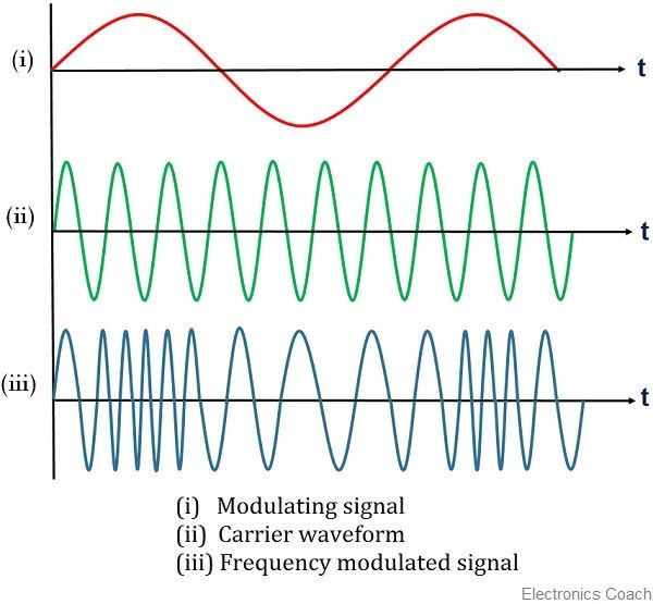
There are a few different types of modulation, but if you are a FM broadcast radio station, you will be using frequency modulation (yes, this is where the acronym FM comes from). While the theory behind this process is interesting, for our purposes it is largely unimportant. If you so desire, you can read more about it here. As its name suggests, frequency modulation changes the frequencies of the carrier wave to have the information from our audio signal without distorting it is amplitude. In the figure shown below, the low frequency audio wave, shown in red, is frequency modulated onto the higher frequency green wave. The resulting blue colour wave is what gets transmitted out.
How does an FM radio stations choose a carrier wave? Each FM broadcast station is assigned one of a hundred different carrier wave. These waves range from 88.1 MHz to 107.9 MHz in 200 kHz intervals. So if you tune your radio to FM 99.99, you will be listening to the FM radio station that is using a carrier wave of 99.9 MHz. Finally FM Receivers, like the one we will build today, take the incoming FM signal and demodulate them to get an audible wave.
Setting up a new gnuradio project
Software defined radios take the analog signals processing and move as much of it into computer algorithms using software as possible. Most of the time, we want our algorithms to be maintainable and performant, so we write them in a language like C++. However when we are trying to prototype something quickly to ensure that the hardware is working, your probably not going to end up writing code that is maintainable or performant. gnuradio is a graphical tool (GUI) that we can use to generate code for software defined radios, without having to write any ourselves. It is great for getting started and prototyping your ideas quickly. Each gnuradio project is a flow graph composed of blocks that represent different signal processing functions. These graphs run from source blocks that sample incoming waves to sink blocks that convey the output of our processing (for example as a waterfall graph or as a audio output).
Go ahead and start a new project. At first you should have two blocks: an Options and a Variable block. These two blocks are separate from the flow graph that we will use for our FM receiver algorithm, but are still part of the gnuradio project. Clicking on the block will give you a dialogue box that will let you modify it.

In the Options block you will want to set the ID, Title, Author and Description fields. Once we start to run our flow, gnuradio will generate some python code. The ID field will become the name of the python file so make sure you name it using snake case.

The Crimson TNG / Cyan can handle a higher sample rate than the default so go ahead and change the Variable Block to 1e6 (This is a concise way to represent 10^6 = 1 000 000, think scientific notation). One way to do this is to click on the box like we did before, but another option is to use the variable editor (shown below). If you cannot see this, make sure the option is checked under the view menu.

Connection types
When our initial wave form is sampled, the software uses quadrature signals that form a stream of complex numbers. The exact math behind this technique is not so important, but it does have one important implication: sometimes our sampled points will be complex, other times it will be floats. When connecting blocks together, we will need to make sure that the connection types line up properly.
Before we start hooking things up, let me provide an overview of the blocks that we will use and their connection types. The table below shows the input and output types that we will be using for each of the blocks in our project.
| Block | Input Type | Output type |
|---|---|---|
| UHD USRP Source | none | complex |
| QT GUI Time Sink | complex | none |
| QT GUI Frequency Sink | complex | none |
| QT GUI Waterfall Sink | complex | none |
| Audio Sink | float | none |
At first, we will be able to use the complex connection for all the blocks. Once we start to bring in the audio sink, we will use a Complex to Float block to ensure that it can receive our signal.
Hooking up the radio
Let us get started! We can create our first flow graph by hooking up our source block to the three graphical blocks: QT GUI Frequency, QT GUI Time Sink and QT GUI Waterfall Sink. You can join blocks by clicking on them one after another:

You should now be able to generate code and run it as is!
Using Separate tabs for separate sinks
To make the graphs more readable, we can create Tabs for each one. You can create tabs by setting the labels in a QT GUI Tab Widget and then adding tabs@<label number> on each sink. For example, if we set Label 0 to Time Sink, then we will want to set the GUI hint in the Time Sink’s block to tabs@0.
Setting the RF Options
Instead of specifying the station with a regular variable, let us use a slider that we can interact with.
Now let us create a slider that we will be able to use to set the radio station. To create a slider use the QT GUI Range block. How do you know what values your slider should have? Refer back to the section on background and terminology.
| Field | Value |
|---|---|
| id | station |
| Default Value | 99.9 (or any radio station that you know in your area with a strong signal) |
| Start | 88.8 |
| Stop | 197.9 |
| Step | 200e-3 |

Next, we will need to convert the value from the slider to a frequency that we can use to set our receiver. I created a new variable called center_freq and set it to station * 1e6 (since the frequency of our carrier wave is in MHz). Once we have the center_freq value, we can set it in our source uhd block. You will also need to set the gain. You can do this directly, or create a separate variable for it.

Warning
Before we start to bring in the audio sink; now is a good time to double check that you have an antenna plugged into the RxA port of the Crimson TNG/Cyan.
Audio Sinks
If we are building an FM Receiver, we probably want some way to listen to our output. For that we will need an Audio sink. In the radio documentation it recommends that for typical applications, the sampling rate should be set to 48kHz, so let us change that and run with the other defaults!
Since the Audio block can only receive floats, you will need a Complex to Float block to get it working. The converter block has two outputs. The top one is the real portion and the bottom half is the imaginary portion. Make sure you only use the top half.

Create a new variable called vol and Connect the Complex to Float block in series to a Multiply Const with the new vol variable as the constant. Connect the output of the Multiply Const block to the Audio block.
The plots that we have so far, provide us with immense detail. But in this case it is going to be easier to see if things are on the right track by listening to the output.
Note
The audio block uses pulse audio on Linux machines. I faced some trouble trying to get the audio to work over an ssh connection. I eventually resorted to using a speaker on the remote machine directly.
Decimating our samples
Go ahead and compile the code as we have it now. When you run it, you should hear static, if you cannot you can raise the vol variable to turn up the volume.The reason we can only hear static is because our sample rate is too high at the output of our flow. To fix this problem, we can “downsample” our incoming wave.
We can do this by making use of the Decimate field of the Rational Resampler block. Create a variable for the decimation amount and fiddle around with a few different values to see what works (if it works well, you should only hear solid static). I called the variable rr_decim and found that setting it to 5 worked well.

Note
Our effective sampling rate is now incoming_sampling_rate / rr_decim, which is slower than what we had before. This is also sometimes called the Channel Rate.
As you can probably guess, the Rational Resampler belongs directly after the UHD Source block. At this point, our flow should look something like this:

FM Demodulation
Now for the crux of our FM receiver, the demodulator. For this, we will use the “FM Demod” block.
| field | variable | value |
|---|---|---|
| Channel Rate | channel_rate |
samp_rate / rr_decim |
| Audio Decimation | fm_decimate |
4 |
| Deviation | deviation |
150e3 |

For reasons that we will not discuss here, there is some wiggle room around carrier signal that the radio station emits. The max FM broadcasting deviation is 75kHz on either side of the carrier signal. Since FM stations are spaced at 200 kHz intervals, this leaves a 50 kHz buffer between each FM radio station. This is also the reason why you can still hear FM 99.9 if you tune your radio to 99.8, but only get static if you tune your radio to FM 100.00 MHz.
Since our audio sink is sampling at a rate of 48kHz, we will want to try and get our sample rate as close to that as possible. (200kHz / 48kHz ~= 4 which is what we use for fm_decimate)
Connect the output of the “FM Demod” block to a Multiply Const block with a value of 1. Change the “type” fields of QT GUI Frequency, QT GUI Time Sink and QT GUI Waterfall Sink from complex to real.
Adjusting the Volume
The final wave that we hear is a sound wave. The amplitude of a sound wave is its intensity, which is what the human ear perceives as volume. If we multiplied the final audio wave by 0.5 , we would end up with a wave that is only half as loud and if we wanted to mute the radio completely, we can multiply the wave by 0. If we wanted to create a volume slider that has the values 0 - 10, we just have to map them to fractions that we can multiply the original wave by. The most straightforward way to do this is to multiply our outgoing signal by 0.1 times the selected volume.
The final product
Here is what your final FM Receiver should looks like:

And when you compile and run it, you should be able to see the generate graphs and hear the audio output.

Congrats! You have now setup an FM broadcast receiver. Next time, we will try and do this all in code!
Additional Resources
- If you want to apply parts of this tutorial to other Software Defined Radios, check this out
- Some good non-technical explanations of modulation and frequency modulation
- If you are looking for more technical detail, consider looking here
- If you want to learn more about the technical and legal requirements of operating an FM radio station in Canada, look here